Errors and Error Correction in the Quantum World

To err is human. Sadly, computers do that too. Classical computers play around with a multitude of bits at any point in time. It is not hard for a noisy environment to flip random bits here and there. A single bit flip can lead to a tsunami of errors in calculations; multiple bit flips can be devastating. Fortunately, modern-day computers handle these errors quite well, and we have elegant error-correcting codes (ECCs) at hand. Redundancy is at the heart of such error-correcting codes. Let us see how:

A crude way of detecting and correcting bit-flip errors is to encode $ [0, 1] $ as $ [000, 111] $. We have created multiple copies of the same bit. Here, 3 bits constitute one logical bit or codeword. Any single bit flip can now be easily corrected by selecting the value of the majority of the bits. Let’s say our data is the binary sequence $ 0 1 0 $. It can be encoded as $ 000\ 111\ 000 $. Now, even if some random bits flip due to errors, $ 010\ 110\ 100 $, we can always correct the errors by choosing the value of the majority of the bits, taken in threes. $ 010 $ is corrected to $ 000 $, $ 110 $ to $ 111 $ and $ 100 $ to $ 000 $. Therefore, $ 010\ 110\ 100 $ is corrected to $ 000\ 111\ 000 $, which can be decoded back to $ 0 1 0 $, the original binary sequence.

The Quantum Realm

Things get pretty tricky as we enter the quantum realm. It is essential to understand what a qubit is, in order to understand quantum errors. A qubit (short for quantum-bit) is a two-level quantum system used as a basic unit of information in quantum computing. The state of a qubit is represented by vectors (or wave functions). A qubit can have states $ \vert 0⟩ $ and $ \vert 1⟩ $ (analogous to 0 and 1 in classical bits). The brackets around $ \vert 0⟩ $ and $ \vert 1⟩ $ are a fancy way of representing vectors in a notation called the Dirac notation. The symbol $ \vert ψ⟩ $ is generally used to represent the state of a qubit.

Two interesting phenomena that set the qubits apart from classical bits are superposition and entanglement. Superposition allows a qubit to achieve states which are a linear combination of $ \vert 0⟩ $ and $ \vert 1⟩ $, i.e. $ c_1\vert 0⟩+ c_2\vert 1⟩ $ (where $ c_1, c_2 $ are complex numbers and $ \vert c_1\vert ^2+ \vert c_2\vert ^2 = 1 $). A qubit can therefore choose from an infinite set of states, taking arbitrary values of $ c_1 $ and $ c_2 $. Entanglement is the name given to a strong correlation that can exist between two or more qubits. It is amusingly called “spooky action at a distance” since the correlation is independent of the separation between the qubits. Both superposition and entanglement are essential tools in many quantum algorithms. Geometrically, a qubit is neatly represented as a point on (or inside, but that’s a topic for another day) a special unit sphere known as the Bloch Sphere:


The Bloch Sphere visualized, ¹

The state of the qubit is re-parameterized in terms of $ θ $ and $ φ $ to fit on the Bloch Sphere.

\Large \vert ψ⟩= e^{iγ} (\cos{\dfrac{θ}{2}} \vert 0⟩+ e^{iφ} \sin{\dfrac{θ}{2}} \vert 1⟩)

$ e^{iγ} $ represents the global phase factor and has no effect on the Bloch Sphere representation of the qubit.

Errors

All quantum algorithms are developed considering qubits to be perfectly isolated from the environment. However, a perfectly isolated quantum system is realistically impossible to achieve. We strive to achieve near-perfection, but the system essentially remains an open system. Open quantum systems interact with the environment and exchange energy. This interaction is the root cause of quantum errors. The Hamiltonian of the interaction decides the type of error that occurs. A Hamiltonian is nothing but an operator that describes the energy of the quantum system.

An easy way to look at quantum errors is in the form of deformities of the Bloch Sphere. The type of deformation depends on the Hamiltonian of the interaction. Let us look at some single qubit errors:

Phase-flip error

We represented a qubit as $\vert ψ⟩= e^{iγ} (\cos{\dfrac{θ}{2}} \vert 0⟩+ e^{iφ} \sin{\dfrac{θ}{2}} \vert 1⟩)$ The term $ e^{iγ} $ is called the global phase of the qubit. A qubit is represented by the same point on the Bloch Sphere, irrespective of the global phase. However, when the qubit is in a superposition, the relative phases of different states cannot be ignored. For example, a qubit in state $ -\vert 1⟩ $ is indistinguishable from a qubit in state $ \vert 1⟩ $. However, a qubit in a superposition $\vert +⟩ = \dfrac{1}{\sqrt{2}} (\vert 0⟩ + \vert 1⟩)$ is different from $\vert -⟩ = \dfrac{1}{\sqrt{2}} (\vert 0⟩ - \vert 1⟩)$ $ \vert +⟩ $ is represented along the positive $ X $ axis, whereas $ \vert -⟩ $ is represented along the negative $ X $ axis. The phase-flip error is similar to applying a $ Z $ gate on the qubits. A $ Z $ gate changes a qubit state $ \vert 1⟩ $ to $ -\vert 1⟩ $ but it has no effect on the state $ \vert 0⟩ $. Therefore, under a phase-flip error, a qubit starting in state $c_1\vert 0⟩ + c_2\vert 1⟩$ starts oscillating between the states $c_1\vert 0⟩ + c_2\vert 1⟩ \text{ and } c_1\vert 0⟩ - c_2\vert 1⟩$ On an average, it can be visualized as the shrinking of the $ XY $ plane of the Bloch Sphere:


Phase Flip Error

Bit-flip error

A bit flip error is an error in which the state $ \vert 0⟩ $ of the qubit is flipped to $ \vert 1⟩ $ and vice-versa. The error can be simulated by the application of a X gate on the qubits. Thus, a qubit starting in the state $c_1\vert 0⟩ + c_2\vert 1⟩$ starts oscillating between the states $c_1\vert 0⟩ + c_2\vert 1⟩ \text{ and } c_1\vert 1⟩ + c_2\vert 0⟩$ On an average, it can be visualized as the shrinking of the $ YZ $ plane of the Bloch Sphere.

Bit-phase flip error

A bit-phase flip error combines bit-flip and phase-flip errors and can be seen as applying a $ Y $ gate on the qubits. $ Y $ gate changes a qubit in state $ \vert 0⟩ $ to state $ i\vert 1⟩ $ and a qubit in state $ \vert 1⟩ $ to state $ -i\vert 0⟩$ . Thus, a qubit starting in the state $c_1\vert 0⟩ + c_\vert 1⟩$ starts oscillating between the states $c_1\vert 0⟩ + c_2\vert 1⟩ \text{ and } ic_1\vert 1⟩ - ic_2\vert 0⟩$ On an average, it can be visualized as the shrinking of the $ XZ $ plane of the Bloch Sphere.

Depolarization

In depolarization, there is uniform shrinking of the Bloch Sphere. Eventually, the state shrinks to a point at the center of the Bloch Sphere, and all information is lost.


Depolarization

Spontaneous emission

The state $ \vert 0⟩ $ is naturally a lower energy state than state $ \vert 1⟩ $. In spontaneous emission, the qubit emits energy to the environment and slowly recedes towards the lower energy state $ \vert 0⟩ $. This happens when the environment is at absolute zero, such that the qubit only emits energy to the environment and no energy is absorbed from the environment.


Spontaneous Emission

Spontaneous emission + thermalization

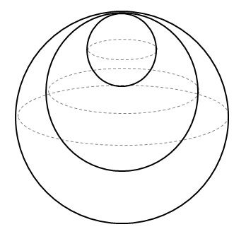
More realistically, when the environment is at temperatures above absolute zero, the qubit emits energy to the environment and also absorbs some energy from the environment. In this case, the Bloch Sphere recedes to a point P of minimum energy inside it. This is termed spontaneous emission + thermalization.


Receeding Bloch Sphere

Challenges in Error Correction

Continuum of errors

Intuitively, any slight nudge to the state of a qubit represented on the Bloch Sphere can be characterized as a quantum error. A correct state of a qubit has infinite possibilities to choose from in the error subspace. We have to deal with a continuum of quantum errors!

No-Cloning Theorem

Remember how we talked about redundancy being at the heart of classical error-correcting codes? Things get spicy in the quantum realm, thanks to the no-cloning theorem. The no-cloning states that it is impossible to create an independent and identical copy of an arbitrary unknown qubit state. We have to come up with ways to create redundancy without cloning the state of a qubit!

The collapse of the wavefunction

The measurement postulate of quantum mechanics states that the state of a qubit collapses upon measurement. This translates to the destruction of the qubit, and hence information, once a qubit is measured. We have to develop ways to look for errors and correct them without measuring the qubit!

Overcoming the Challenges

The proposed challenges might make it look impossible to design error-correcting codes for quantum systems. However, humans are smart. We have some neat tricks to overcome the proposed challenges. Understanding the following section requires some background knowledge about qubits, quantum gates, and quantum circuits.

Digitization of errors

An open quantum system evolves according to the following equation:

\Large ρ_{new} = \sum (K_{\alpha} \ ρ_{old} \ K^{\dagger}_{\alpha})

$ ρ $ is the density operator, which is an alternate way of representing the state of a qubit. $ K_{\alpha} $ is the Kraus operator that satisfies the property: $\sum (K_{\alpha}\ K^{\dagger}_{\alpha}) = 1$ Each state that is a part of the density operator ρ evolves as follows: $\vert ψ⟩_{new} = K_{\alpha} \vert ψ⟩_{old}$ $ K_{\alpha} $ can be represented as a $ 2 $ x $ 2 $ complex matrix. The identity matrix and the Pauli matrices : ${\hat{I}, \hat{σ_x}, \hat{σ_y}, \hat{σ_z}}$ form the basis for $ 2 $ x $ 2 $ complex matrices over complex numbers.


Pauli spin matrices

The Kraus operator can be expressed in terms of the basis matrices as:

$K_{\alpha} = \alpha_i\hat{I} +\alpha_x\hat{σ_x}, +\alpha_y\hat{σ_y}, +\alpha_z\hat{σ_z},$ where $ \alpha_i $, $ \alpha_x $, $ \alpha_y $ and $ \alpha_z $ are arbitrary complex numbers. An interesting property of the Pauli matrices is that $ i\hat{σ_x}\hat{σ_z} = \hat{σ_y} $. Therefore, the Kraus operator can be reformulated as $K_{\alpha} = \alpha_i\hat{I} +\alpha_x\hat{σ_x}, +\alpha_y i\hat{σ_x}\hat{σ_z}, +\alpha_z\hat{σ_z}$ . The beauty of this reformulation is that we have mapped general noise to discrete Pauli errors using a bit of mathematics. We have to correct only Pauli X and Pauli Z errors. We have immensely narrowed down the class of errors that we have to deal with. We no longer have to address the continuum of errors.

Entanglement for redundancy

The no-cloning prevents us from creating exact independent copies of an arbitrary unknown state, but we can create redundancies using the power of entanglement. We can easily create an entanglement using the C-NOT gates as shown:


C-NOT gates

Here, if $ q_0 = c_1 \vert 0⟩+ c_2 \vert 1⟩ $, $ q_1 = \vert 0⟩ $ and $ q_2= \vert 0⟩ $, the outcome of the circuit is simply $ c_1 \vert 000⟩+ c_2 \vert 111⟩ $. Voila! We have achieved redundancy without violating the no-cloning theorem here. Cloning a state $ c_1 \vert 0⟩+ c_2 \vert 1⟩ $ would mean creating three independent copies of it. What we have created is an entanglement of three qubits, due to which the three qubits are dependent on each other. However, these entangled qubits are good enough for our purpose.

Projective measurements

When a qubit $ c_1 \vert 0⟩+ c_2 \vert 1⟩ $ is encoded to $ c_1 \vert 000⟩+ c_2 \vert 111⟩ $, we have expanded the state space of qubits from a 2-dimensional state space to an 8-dimensional state space. The 8-dimensional state can be thought of to be composed of a logical qubit subspace with ${\vert 000⟩, \vert 111⟩}$ as the basis and an error subspace with ${\vert 001⟩, \vert 010⟩, \vert 011⟩, \vert 100⟩, \vert 101⟩, \vert 110⟩}$ as the basis. A correct qubit always resides in the logical qubit subspace. It is only when errors occur that the qubit goes to the error subspace. For example, a correct qubit $ c_1 \vert 000⟩+ c_2 \vert 111⟩ $ in the logical qubit subspace may be changed to $ c_1 \vert 010⟩+ c_2 \vert 110⟩ $ due to errors, thereby entering the error subspace.


Logical Qubit subspace and error subspace

To avoid the destruction of the state of the qubits due to measurement, we make use of an extra qubit called an ancillary qubit. We measure only the ancillary qubit, leaving the other qubits undisturbed. We model the quantum circuit such that the measurements of the ancillary qubit help to detect whether our qubits are in the logical qubit subspace or the error subspace.

The Quantum Threshold Theorem

The quantum threshold theorem says that a quantum computer with a physical error rate below a certain threshold can, through application of quantum error correcting schemes, suppress the logical error rate to arbitrarily low levels. There was a time when it was considered unrealistic to create real world quantum computers due to the challenges posed by quantum errors. However, using the techniques described above as the foundation, elegant error correcting codes have been proposed to detect and correct quantum errors. Shor’s 9 qubit code is a remarkable checkpoint in quantum error correction. It uses nine qubits to encode one logical qubit and is able to correct phase-flip, bit-flip and bit-phase flip errors! Quantum error correction is an active area of research that re-establishes our faith in the creation of feasible quantum computers in the near future.